Getting Started¶

This page takes you from a fresh install to a predictor running on your own Gymnasium environment. ppsds has two sides: a floor (the conic DRPP predictor) and a ceiling (how well anything could predict a system known exactly). This page puts the floor on your system; the ceiling is one section below. The path is short (you declare three things and run a loop), but one precondition is worth stating before anything else.

The guarantee has a precondition: the ambiguity set you declare must contain the true system. ppsds is not "install it and the predictions get better". It is "state what you are uncertain about, and get a worst-case lower bound on the score". Declare too little and the bound is vacuous; declare too much and the predictions are needlessly conservative. Choosing those declarations is the whole job; see Preliminaries for what the predictors actually optimize.

Install¶

pip install ppsds

0.0.3-alpha is a pre-release: pin it with pip install ppsds==0.0.3a0, or pass --pre.

To run the examples in this repository, install from a checkout instead, so the editable ppsds resolves to the tree you are reading:

git clone https://github.com/Xuzerken/ppsds
cd ppsds
pip install -e ".[experiments]"     # `experiments` adds matplotlib/pandas/seaborn/tqdm for the figures

The core needs only numpy, scipy, cvxpy and gymnasium, and Python 3.10 or newer. The README has the full dependency split; the short version is that the predictors and ppsds.environment are core, while ppsds.experiment and ppsds.visualization sit behind the optional experiments extra.

The smallest thing that runs¶

python examples/apply_drpp_to_your_own_env/quickstart.py

About one second, 50 steps, on a two-state system that stands in for "your own environment":

Running 50 steps on **one ordinary trajectory** (your own environment, zero control)

predictor     mean log score   note
----------------------------------------------------------------
nominal               -2.867   trusts the nominal model
Eig-DRPP              -3.366   made robust to the worst case

Read the two numbers as a pair. nominal scores higher here, and that is the normal case, not a bug; see the first pitfall below. The real content of the example is the shape of the workflow: the environment is only ever stepped, the predictors take their model from an ambiguity set you declared, and each score is computed against the state that actually arrived.

Putting it on your own environment¶

Section 0 of quickstart.py is a stand-in environment; everything after it is what you actually write. You do not modify the environment. You declare three things, and the order matters:

import numpy as np
from ppsds.ambiguity.additive_drift.conic_moment import LinearAmbiguitySet
from ppsds.probabilistic_predictor.drpp.additive_drift.conic_moment import (
    NominalPredictor, EigDrpp,
)
from ppsds.scoring_rule.logarithm_score import LogarithmScore

# (1) The nominal model -- "what I believe my system is".
#     Independent of which family you pick: changing family does not touch this.
A_bar = np.array([[1.0, 0.10], [0.0, 1.0]])
B_bar = np.array([[1.0], [0.0]])
mu_bar = np.zeros(2)
Sigma_bar = np.array([[1.0, 0.45], [0.45, 1.30]])

# (2) Fix the **family** of the ambiguity set first. Different families describe uncertainty
#     in completely different languages, so this decides what step (3) has to supply.

# (3) Within that family, declare its parameterization.
alphas = {'A': 0.30, 'B': 0.30, 'mu': 0.25, 'Sigma': 3.0}
f_err_max = 0.30
abg = LinearAmbiguitySet(A_bar, B_bar, mu_bar, Sigma_bar, alphas, f_err_max)

# (4) The predictors take their model from the ambiguity set -- do not retype the literals,
#     or "the model the predictor uses" and "the model the set declares" drift apart.
predictors = {
    'nominal':  NominalPredictor(abg.f_bar, abg.mu_bar, abg.Sigma_bar),
    'Eig-DRPP': EigDrpp(abg.f_bar, abg.mu_bar, abg.Sigma_bar, abg.gamma),
}
scorer = LogarithmScore()

x, _ = env.reset(seed=0)                     # `env` is yours; DRPP never needs to modify it
for _ in range(50):
    u = policy(x)
    for pred in predictors.values():
        pred.update(x, u)                    # update from the current observation
    x, *_ = env.step(u)
    for name, pred in predictors.items():
        score = scorer.score(pred.predict(), x)

The one line that is easy to get wrong is the timing: the predictors are updated from (x, u) before env.step(u), and the prediction just issued is scored against the state that comes back. ppsds never asks the environment for anything, so nothing about your environment has to change to fit it.

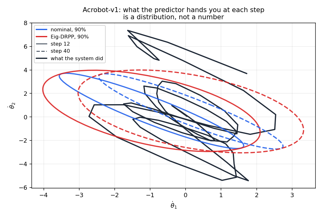
The true trajectory through one plane of Acrobot's state space, with the 90% predictive distribution at two steps: nominal in blue, Eig-DRPP in red, and the robust one visibly wider

What the floor is worth, and when it pays¶

Before you commit to the robust predictor, look at what it actually buys. The figure below is the same off-the-shelf environment (Acrobot-v1) scored with a nominal model identified from different amounts of data. The model is bad in every column — that never changes. What changes is whether the noise you declared was too narrow:

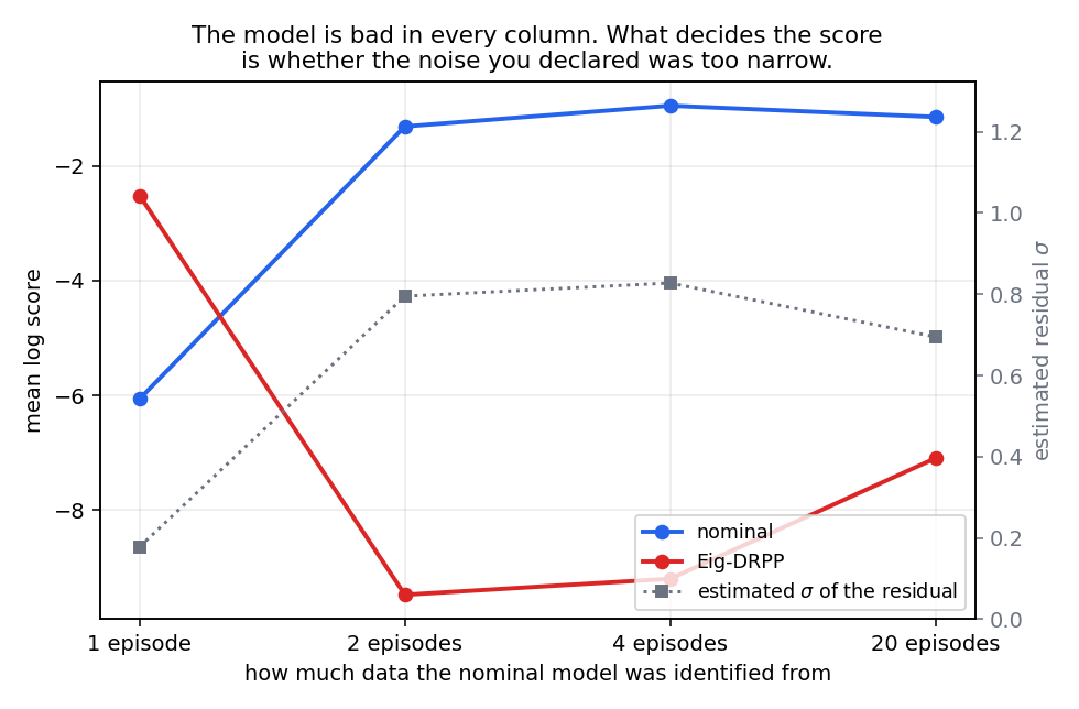
Mean log score of the nominal and robust predictors, against the estimated residual standard deviation, as the identification data grows from one episode to twenty

With one episode the residual is badly underestimated, Sigma_bar comes out far too narrow, and the nominal predictor scores terribly on the errors it meets — while the robust one holds.
With more data the estimate is calibrated, the nominal predictor wins, and DRPP's robustness is pure insurance premium.

So the decision is not "how good is my model" but "how confident am I in my own declaration" — and too little identification data is the most common source of misplaced confidence. The apply_drpp_to_your_own_env example runs the whole comparison and prints the table these two figures are drawn from.

If you do not know a nominal model¶

If your environment has no analytic dynamics, identify a linear model from rollouts first:

from ppsds.dynamics.identification import collect_rollouts, fit_linear, diagnose, format_report

X, U, X_next = collect_rollouts(env, policy, n_episodes=20, T=200)
fit = fit_linear(X, U, X_next)          # x' ~= A x + B u + c
res = fit.residuals(X, U, X_next)
print(format_report(diagnose(res, X_next - X), fit))

That report tells you how large the residual is, whether it still has lag-1 structure, and whether its covariance is numerically singular: the numbers your declarations should be based on. The Acrobot and Pendulum examples do exactly this, and their output is on the Examples page.

The other side: the ceiling¶

The floor is not the only question. For a system you know exactly, there is a number that no predictor can beat: the probabilistic predictability. Computing it needs no predictor and no optimization, because it is a property of the system, not of a method.

python examples/understand_predictability/quickstart.py     # about two seconds

It prints six golden values you can check against the formula, then compares them with a predictor over ten thousand trajectories. The whole experiment runs in seconds; that contrast is the point. If you are comparing predictors, this is the reference line they are measured against, and it is also the upper bound that makes the DRPP floor meaningful.

The definition and the bound: probabilistic predictability paper
The example: the ceiling
The paper-scale figure: the predictability experiment

Common pitfalls¶

1. On an ordinary trajectory, DRPP scores lower than nominal, and that is expected. The example above shows it. DRPP trades average performance for a worst-case floor; on a trajectory where your declaration happens to be about right, the conservatism is pure cost. What makes DRPP win is not a bad model but an optimistic declaration (pitfall 4).

2. The conic-moment radii mix squared and un-squared quantities. This is the easiest place to be off by a square:

quantity	convention
`f_err_max`	un-squared: \(\lVert\delta_f\rVert \le \texttt{f\_err\_max}\)
`alphas['mu']`	squared: \(\lVert\mu-\bar\mu\rVert \le \sqrt{\alpha_\mu}\)
`alphas['Sigma']`	scaling: the true covariance is dominated by \(\alpha_\Sigma \bar\Sigma\)
`alphas['A']`, `alphas['B']`	un-squared: the largest perturbation of the corresponding entry

f_err(x, u) (also exposed as gamma[0]) is the odd one out: the callable returns a squared bound, while f_err_max is the un-squared hard bound. Their magnitudes set the magnitude of the score, so they are not numbers to guess: take them from physics (unobserved perturbations, actuator and sensor noise, unmodelled high-frequency dynamics), or from a first run whose magnitude you check against your intuition for "how accurate the prediction should be".

3. A deterministic environment has no noise to measure, and its residual covariance is often structurally singular. Most classic gymnasium environments return bit-identical results for the same state and action. That is not a defect: the model is a statement about what you believe, and a deterministic environment simply means the noise is entirely unmodelled. The trap is downstream. A covariance estimated from such residuals is often singular, the logarithmic score requires the predictive distribution to have a density, and a degenerate distribution scores -inf for almost every value. You must regularize, and the size of that regularization is itself a modelling decision, because it sets the width of the predictive distribution and hence the score.

4. Too little identification data is the usual reason DRPP wins. Fit Sigma_bar from a small sample and it comes out underestimated: the nominal prediction is too narrow and its score collapses on the errors that actually occur, while Eig-DRPP's covariance already accounts for them. Measured on Acrobot, one identification episode underestimates the residual standard deviation by about 3.9x, and there DRPP wins; with twenty episodes the estimate is calibrated and nominal wins. Whether to reach for DRPP therefore depends on your confidence in your own declaration, not on how accurate the model is. with_standard_gym_env.py prints both regimes side by side.

Pitfalls 5–7 apply to the DRPP experiment (experiments/drpp/).

5. A small -t changes the figures, and says so. The plot indices are fixed in the model table, so a -t below the largest index emits a RuntimeWarning and clamps to the last available trajectory, and the figure content changes accordingly. It no longer crashes (it used to raise IndexError), but the warning is worth reading:

RuntimeWarning: trajectory index in plot_traj 2 out of range (available 0..1); using 1
instead. Note that the figure content changes accordingly; to show a specific trajectory,
raise -t or use a smaller index.

6. The cache is validating, not "the file exists". A completed step is reused only if its recorded fingerprint still matches: source hashes, a parameter snapshot, the sha256 of each dependency, and the array shapes. Change the code or a parameter and it recomputes, telling you why. -f forces everything to recompute; so does a first run over a directory with no manifest.

7. The workers need the fork start method. The nonlinear ambiguity set holds lambdas, so it cannot be pickled. The runner asserts fork and fails loudly rather than degrading silently, so on a platform whose default is spawn (macOS, Windows) you get an explicit message naming the reason instead of a wrong answer.

Platform notes¶

Windows, WSL and Linux are all supported, and every dependency is cross-platform.
Use forward slashes in paths, always: data/gym/traj.pkl, never data\gym\traj.pkl.
Line endings are handled by .gitattributes: content is stored as LF in the repository, shell scripts check out as LF and PowerShell scripts as CRLF. It is the only line-ending guarantee, so leave that file alone.
On Linux, cvxpy (SCS) may need a C toolchain if pip finds no prebuilt wheel; install gcc if a source build fails.

Next¶

I want to...	read
understand the vocabulary and the two pairs of bounds	Preliminaries
see every example, with its command and its real output	Examples
add your own family of ambiguity sets and its DRPP	A new family and its DRPP
see what no predictor can beat on a known system	probabilistic predictability paper
look up a class or function	API

Also in the repository: CONTRIBUTING.md and the issue tracker.